 Aina Frau-Pascual
I am a research scientist with an interest in signal processing, machine learning and data analysis in healthcare, with experience in brain imaging research
Aina Frau-Pascual
I am a research scientist with an interest in signal processing, machine learning and data analysis in healthcare, with experience in brain imaging research
From September 2013 to December 2016, I did my PhD in applied mathematics at Inria and at the Grenoble-Alpes University. I was supervised by Florence FORBES at Inria Grenoble Rhône-Alpes, Mistis (now Statify) team, and by Philippe CIUCIU at Inria Saclay Île-de-France Parietal team, at CEA/Neurospin. I worked on Bayesian methods for the analysis of BOLD and ASL functional MRI data. I was particularly interested in the study of the hemodynamic and perfusion responses due to evoked activity and in the potential clinical biomarkers that could derive from the study of these two fMRI modalities. You can find a summary below.
Here you can find my PhD manuscript and the slides used in my PhD defense. A list of publications can be found in Google Scholar.
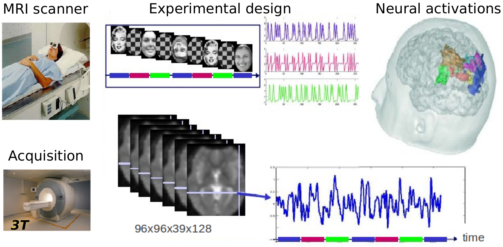
An MR scanner is a huge magnet that records echo signals from tissues -- echoes from signals or radiofrequency pulses generated by the scanner. As a result, it provides images of the brain or the body, that can be like a picture (3D volume) or a video (e.g. 3D volume changing in time). Depending on how we take these images -- how the signals that the scanner emits are designed (we call them pulse sequences) -- the scanner will be sensitive to different characteristics of the tissue and what is highlighted or not in the image, and the color contrasts will vary. You could think of pulse sequences as the lens of a camera, we will focus on some things or others. Depending on the pulse sequence used, the scanner can be sensitive to proton density (T1, T2), changes in oxygenation (functional MRI), water movement (diffusion MRI)...
Functional MRI is the imaging of brain activity while a task is being done. In practice, a person is placed in a scanner and she/he performs an experimental paradigm (a task) while images of the brain are acquired. This experimental paradigm is designed to activate neurons in certain regions of the brain, and we get this measures that are images. These images together make a brain volume video where we capture changes in time. But what are these images? What we actually see is where the blood goes after the activation happens. This is called the BOLD effect: blood oxygen level dependent.
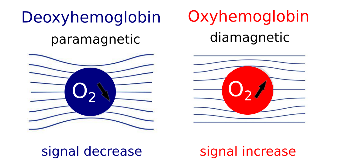
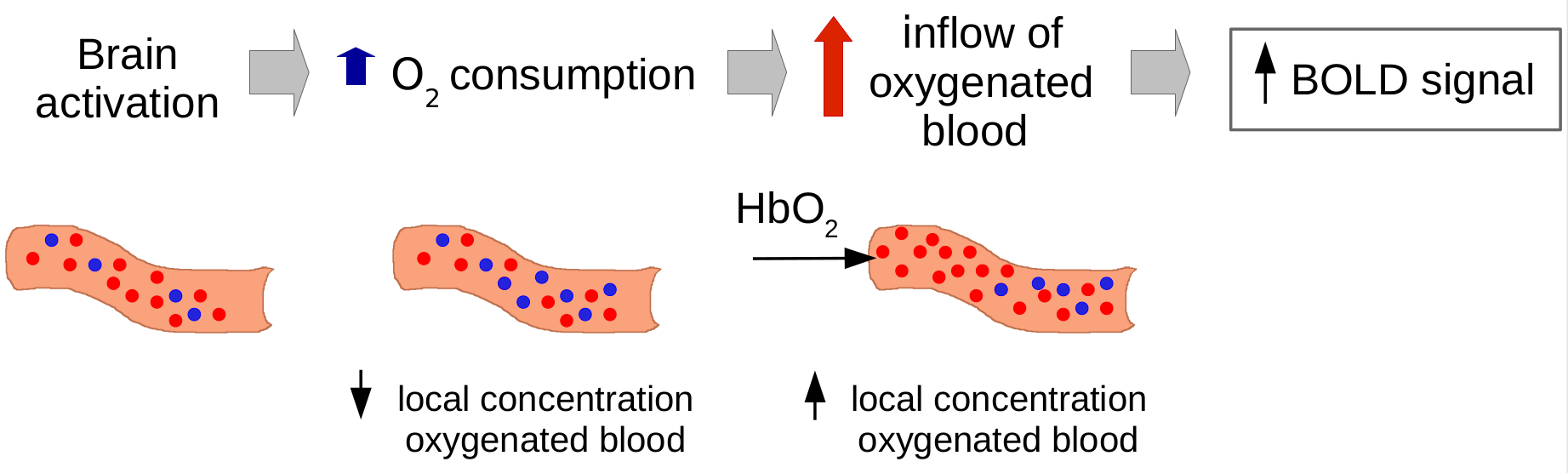
The BOLD effect uses hemoglobin as a natural contrast agent. What BOLD really measures is the ratio of oxy- to deoxy-hemoglobin in the blood because these two states of hemoglobin have different magnetic properties and an increase in deoxyhemoglobin causes a BOLD signal decrease. And when does that happen? When there is brain activity in a certain region, there is a certain oxygen consumption and there is an increase in deoxyhemoglobin. As an effect, there is an inflow of oxygenated blood, which increases the local concentration of oxygenated blood and reduces the percentage of deoxyhemoglobin. This causes a BOLD signal change (~3-4% variation), that we measure as a percentage with respect to baseline. The BOLD effect is an interconnected mix of different changing signals: cerebral blood flow, cerebral blood volume, and oxygen consumption.
While all this is happening, the scanner is acquiring images often -- one every repetition time (TR) -- and we can therefore look at these changes in time, and infer the location of this oxygen consumption effect.
Arterial spin labeling gives us the possibility of measuring cerebral blood flow (CBF) -- the blood coming to the brain through the neck -- specifically and in a quantitative manner. This is important because it is a more direct and precise measure than the BOLD effect. CBF is an important tool for clinicians, because it is typically altered in a number of pathologies: stroke, tumors, dementia, MS... The fact that ASL can be quantified opens possibilities for its use in the clinic and in research (e.g. compare fMRI experiments between and across patients).
To measure CBF directly, pulsed ASL modifies the blood being perfused to the brain through the neck with a magnetic labeling (magnetic inversion). This labeled water molecules reach the capillary bed after some time and cause magnetic disturbances in the local tissue when water molecules from blood and tissue are exchanged. An MRI image is acquired to capture this effect.
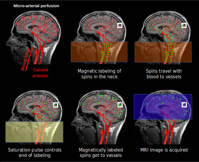
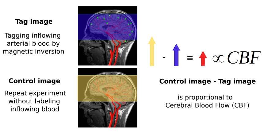
We then need a control image, acquired without labeling inflowing blood, to subtract to the labeled image. The difference image reflects the amount of arterial blood delivered to each voxel within the transit time. The proportion of CBF is about 1% of the baseline CBF. ASL data consists in alternated control and tag images.
Quantified values can be achieved by applying a transformation proposed in the literature, and that considers parameters of the acquisition procedure and a measured relaxed magnetization (another image type).
So in contrast with BOLD, ASL provides a quantitative measure of CBF instead of an indirect absolute measure of a mix of parameters, but it has a lower SNR and therefore lower resolution than BOLD. ASL has been compared to BOLD in the literature, and has been found to have low inter-session variability and to find more localized activity. Compared to other perfusion imaging techniques, as BOLD imaging, ASL is non invasive and non ionizing. The main drawback of ASL with respect to BOLD is the time resolution limitation: ASL needs to wait for the blood to get to the capillary bed and this can not be avoided. BOLD, on the other hand, keeps being pushed to faster acquisition times.
Now that we know what is fMRI, BOLD and ASL, what was my thesis about? I investigated statistical models for the analysis of ASL and BOLD fMRI modalities, with a focus on ASL, because it has a high potential but it is not widely used.
First of all, we derived a signal model for ASL. How did we do it? ASL data is a time series with alternative control and tag images, both with a BOLD component.
The difference image (control - tag) reflects the amount of arterial blood delivered to each voxel within the transit time. The proportion of CBF is about 1% of the baseline CBF.
The addition image (control + tag) gives us a contaminated BOLD effect, with lower resolution than the BOLD images and lower SNR.
In the end, control and tag images have both a BOLD component, the tag image has a negative perfusion component, and the control image has a positive one.
The signal model is a representation of the signal with mathematics, and it reflects the CBF (or perfusion), and BOLD components. For one voxel $j$, there are 2 dynamically changing components that are due to hemodynamic (BOLD) and perfusion changes induced by the stimulation paradigm or task (represented by $X^m$). For each one, we have a response function that describes the behaviour in time and that we consider parcel-wise, and the amplitude of these functions or activaton levels, that are voxel-wise and change depending on the type of stimulus given to the subject, as it is supposed to “light up” the voxel differently. This maps of activation depend on a hidden variable $q$, that encodes activation/non-activation and that account for spatial regularization using a Markov Random Field. The signal has also a fixed perfusion baseline component with $W$ encoding the control/tag alternation, that completes the perfusion component, and noise and drifts. We have pretty good idea of how these responses look like.
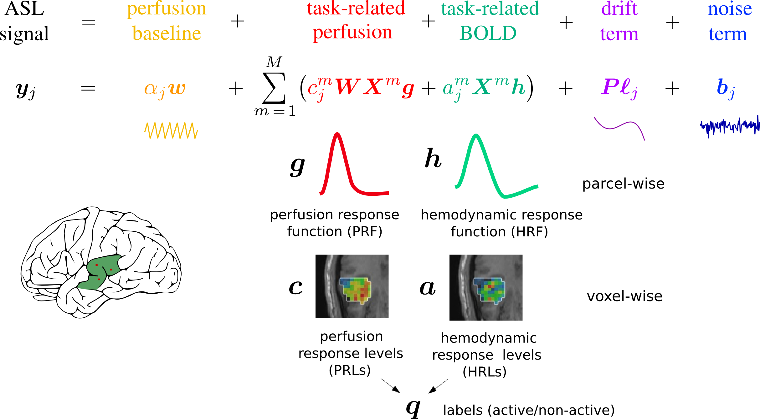
You are probably asking yourself why do we need a signal model and how we are going to use it. In our analysis, we want to separate the different parts of the signal and look at them separately. For example, we can compare temporal patterns in different regions by looking at parameters $h$ and $g$, and we can learn about spatial patterns of task-related activation by looking at parameters $a$ and $c$. Each parameter estimated from the signal model gives us different information about that specific subject's brain.
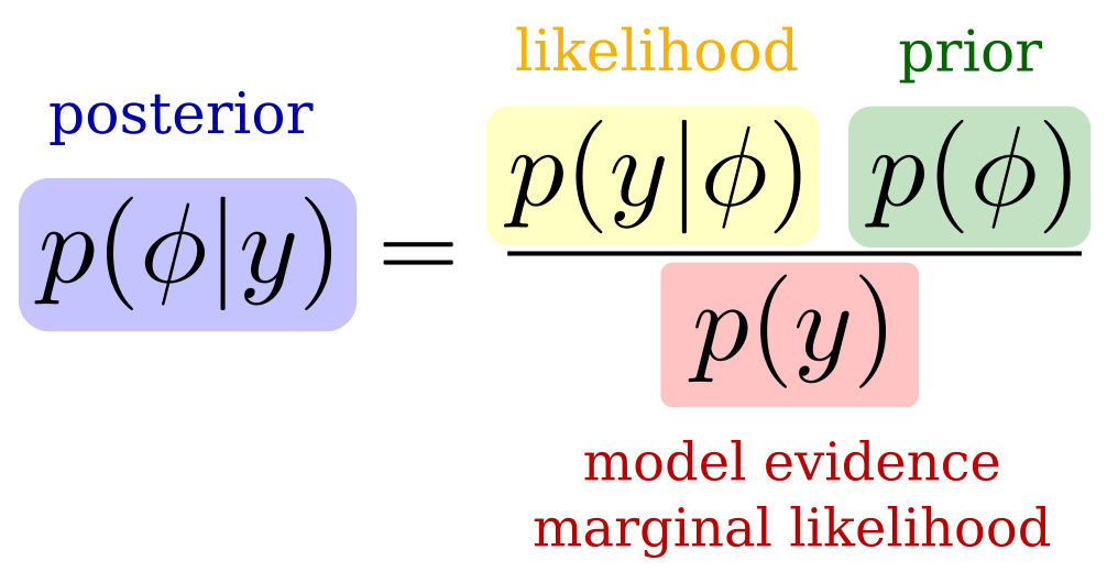
We have many unknown parameters in the signal model. Since we want to be able to estimate the temporal responses, we choose a Bayesian framework to account for prior knowledge on the parameters. In a Bayesian model, we try to estimate the posterior probability function of the parameters from the data or likelihood function and the prior knowledge that we input. The model evidence here is a normalizing constant and it is often intractable.
In our model, we consider parcels and we include several priors:
In a given parcel, we use a prior on the response functions ($h$ and $g$) to enforce temporal regularization. The goal is to get a temporally smooth response function, and we it by including a Gaussian prior with a covariance matrix that enforces this smoothness.
We include priors on the response levels ($a$ and $c$) to enforce spatial regularization. For this, we use a Markov Random Field model, that introduces spatial smoothness.
We include a physiological prior that we derive from physiological models -- Balloon and hemodynamic models -- described in the literature. These models describe the oxygen concentration changes in the blood vessels with a system of differential equations. These equations relate neural stimulus, local blood flow, local capillary volume and concentration of oxygen in the blood. We linearize this system of equations to derive an approximate linear link between the CBF and BOLD responses. This way, we facilitate the estimation of both, but mostly of the CBF response.
We have many different parameters and the posterior is intractable, due to the spatial prior in form of a Markov Random field. For this reason, we need for inference approximation. We can do it with Markov Chain Monte Carlo (MCMC) and Variational Expectation Maximization (VEM) methods. In my PhD, we investigated both solutions but focused on the VEM solution in the end. Although VEM makes an approximation, it reduces the computation cost greatly.
For further information on the derived methods and analysis, check my PhD manuscript.
The validation of the methods was done with the HEROES dataset, a dataset acquired at CEA/Neurospin that has BOLD fMRI, functional ASL (pulsed ASL) and baseline ASL. The measurements that give also access to CBF quantification were also acquired: B1 Mapping and T1 PSSFP with angles 20◦ and 5◦. For the preprocessings, process-asl, a python toolbox that uses nipype and SPM and has been developed at Neurospin, was used.
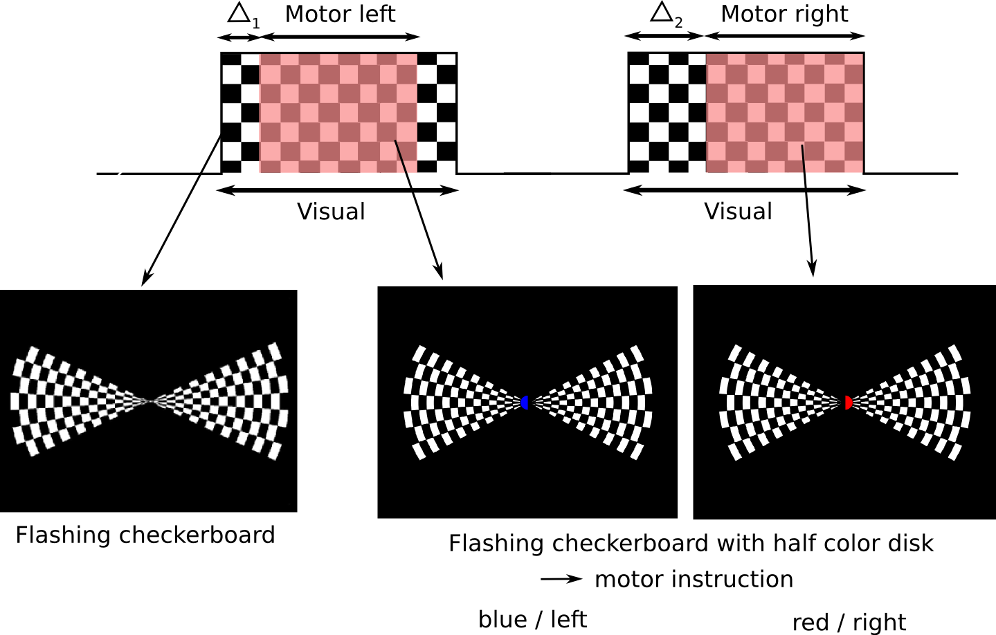
The paradigm combines motor, auditory and visual tasks. The visual task consists in blocks of visual stimulation of 15sec followed by 10sec of rest. The motor tasks are performed during 10sec blocks overlapped with the visual tasks, with different delays. A beep sound is used together with a visual cue to indicate the motor task.
Data was analysed and individual and group results were compared, using Bayesian methods and state of the art methods. ASL and BOLD signal results were also compared giving us some interesting insights and allowing us to validate our methods, which was the goal of this analysis.
Our Bayesian method found higher activation values than state of the art method in BOLD and ASL fMRI modalities.
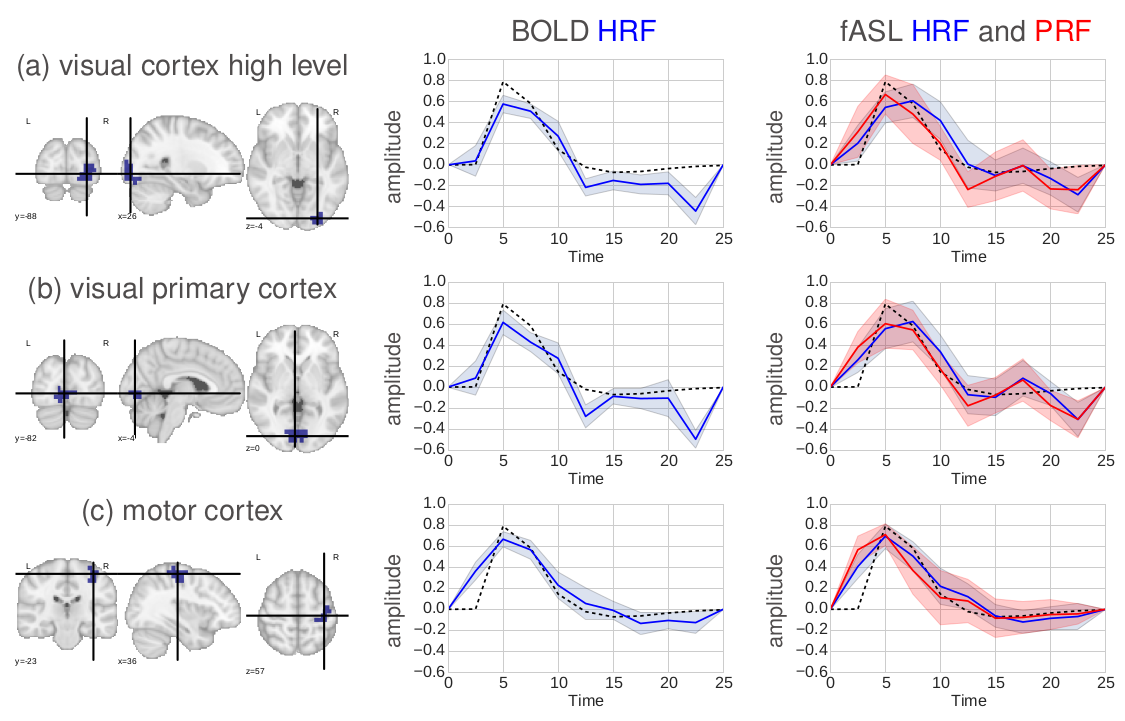
The average temporal responses were similar in BOLD and ASL, and were coherently similar in close regions.
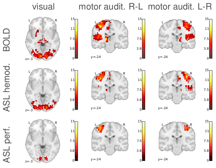
The estimation of temporal responses changed activation detection, finding more activated regions in BOLD, and more localized activated regions in ASL.
The CBF component activation was found to be more localized than the BOLD one, as expected.
Our Bayesian approach was finding higher activation values and also more localized. The use of priors allows for a better modelling of the signal. Specifically, the use of physiological priors was very useful, and the physiological model parameters had to be well tuned to improve convergence of the estimation. However, the interpretation of the activation maps in Bayesian methods and its comparison with state of the art methods becomes challenging. The computation cost of Bayesian methods is also higher than state of the art methods.
ASL provides a more localized activation than BOLD, which makes sense because we are measuring CBF directly. This could be very interesting in the study of brain activity. However, ASL has limitations in terms of resolution and signal to noise ratio. It is a very noisy signal and needs averaging, which is more challenging if you add tasks to the mix. ASL is very useful and already greatly used for resting state (subject not performing any task in the scanner). But probably the biggest challenge for using ASL in task fMRI experiments is its low temporal resolution, which can not be reduced under the time that the blood takes to get from the neck to the capillary bed.